Goodnight
Presenting a slightly different work, but the idea is in line with NLP.
Steps
Step 1: Set up your environment
While we can choose from a number of tools, we’ll walk you through how to set up an IBM account to use a Jupyter Notebook.
Jupyter Notebooks are widely used within data science to combine code, text, images, data visualizations to formulate a well-formed analysis.
Log in to watsonx.ai using your IBM Cloud account.
Create a watsonx.ai project.
Create a Jupyter Notebook.
From here, a notebook environment opens for you to load your data set and copy code from this beginner tutorial
to tackle a simple classification problem.
Step 2: Install and import relevant libraries
We'll need a few libraries for this tutorial. Make sure to import the necessary Python libraries that we need
to work with our Iris data set, perform data preprocessing, and create and evaluate our LDA model. If they're not installed,
you can resolve this with a quick pip install.
import numpy as np
import pandas as pd
import matplotlib.pyplot as plt
import seaborn as sns
from sklearn.preprocessing import LabelEncoder
from sklearn.model_selection import train_test_split
from sklearn.discriminant_analysis import LinearDiscriminantAnalysis
from sklearn.ensemble import RandomForestClassifier
from sklearn.metrics import accuracy_score, confusion_matrix
In this step, we imported essential Python libraries such as NumPy, pandas, Matplotlib, and scikit-learn.
These libraries are crucial for data manipulation, visualization, and machine learning tasks. As a result,
you now have access to the libraries that you need for this tutorial.
Step 3: Read and load the data
In this step, you read the Iris data set from UCI Machine Learning Repository and assign meaningful column names.
The data set contains information about the sepal and petal dimensions of three different species of iris.
url = "https://archive.ics.uci.edu/ml/machine-learning-databases/iris/iris.data"
# Define column names
cls = ['sepal-length', 'sepal-width', 'petal-length', 'petal-width', 'Class']
# Read the data set
dataset = pd.read_csv(url, names=cls)
Step 4: Preprocess the data
In this step, you separate the feature variables (X) and the target variable (y), and encode the target variable y numerically.
# Divide the data set into features (X) and target variable (y)
X = dataset.iloc[:, 0:4].values
y = dataset.iloc[:, 4].values
# Encode the target variable
le = LabelEncoder()
y = le.fit_transform(y)
In this step, we divided the data set into two parts: the independent variables (features, represented as X) and the dependent variable (target class, represented as y). This step involves label encoding which converts class labels into numerical values. The result of this step is a preprocessed data set ready for further analysis.
Step 5: Perform exploratory data analysis
Before you implement LDA, it's essential to analyze the data set and understand its characteristics. In this step, we perform an exploratory analysis of the Iris data set by using a pair plot, histogram, and correlation heatmap.
Pair plots
The pair plot effectively illustrates how the four features vary and correlate across the three classes of iris flowers.
In addition, it provides insights into the separability and overlap of these classes within the feature space,
facilitating a deeper understanding of the characteristics and differences among the classes.
The diagonal plot elements showcase the distribution of each feature, while the off-diagonal plot elements display
scatterplots for each pair of features.
# Create a pair plot to visualize relationships between different features and species.
ax = sns.pairplot(dataset, hue='Class', markers=["o", "s", "D"])
plt.suptitle("Pair Plot of Iris Dataset")
sns.move_legend(
ax, "lower center",
bbox_to_anchor=(.5, 1), ncol=3, title=None, frameon=False)
plt.tight_layout()
plt.show()
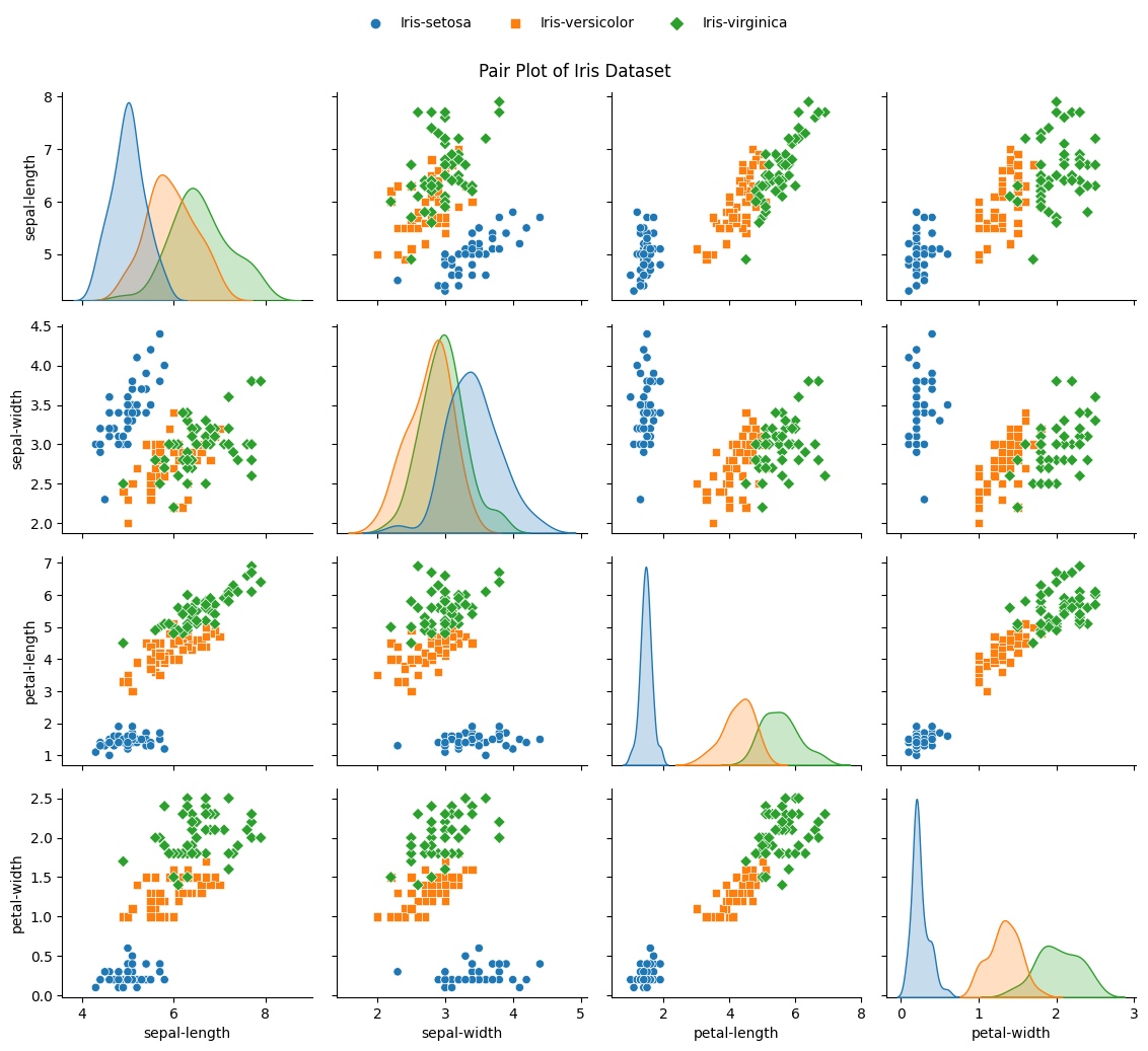
For instance, look at the first column of the plot, which displays the relationship between sepal length and the other features. We can infer the following insights from the pair plot:
The sepal length follows a slightly right-skewed normal distribution.
Iris virginica has the longest sepal length, followed by Iris versicolor and Iris setosa. Iris setosa has the least variation in sepal length, while Iris virginica exhibits the most.
Sepal length negatively correlates with sepal width. Iris setosa has the widest sepal width, followed by Iris versicolor and Iris virginica. Also, Iris setosa is well separated from the other two classes, while Iris versicolor and Iris virginica have some overlap in this feature pair.
Sepal length positively correlates with petal length. Iris virginica has the longest petal length, followed by Iris versicolor and Iris setosa. Here again, Iris setosa is well separated, while versicolor and virginica overlap.
Sepal length positively correlates with petal width. Iris virginica has the widest petal width, followed by Iris versicolor and Iris setosa. Here again, Iris setosa is well-separated, while versicolor and virginica overlap.
You can apply similar analyses to the remaining columns, maintaining this pattern of feature relationships and class distinctions.
Histograms
Histograms are valuable tools for visualizing the distribution of individual features within the Iris data set.
This graph comprises four histograms illustrating the distribution of petal and sepal lengths and widths for the three classes of irises.
# Visualize the distribution of each feature using histograms.
plt.figure(figsize=(12, 6))
for i, feature in enumerate(cls[:-1]):
plt.subplot(2, 2, i + 1)
sns.histplot(data=dataset, x=feature, hue='Class', kde=True)
plt.title(f'{feature} Distribution')
plt.tight_layout()
plt.show()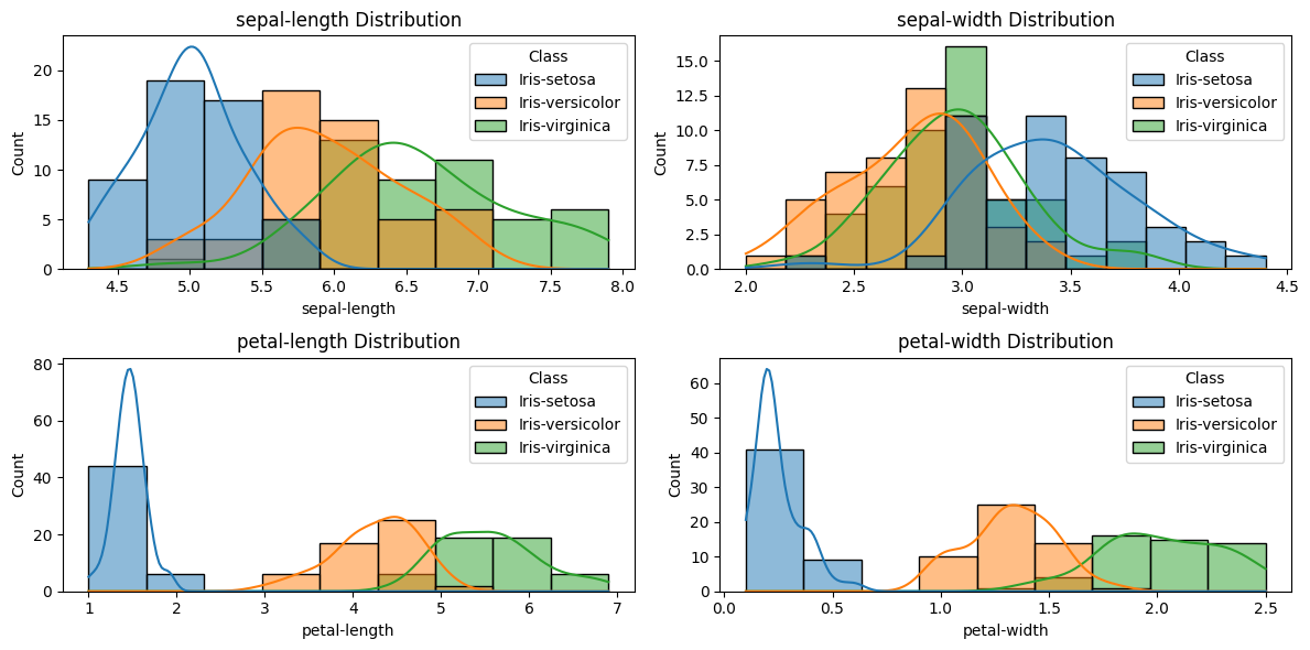
These histograms indicate a balanced data set, but they also showcase the differences among the three classes of iris flowers in terms of petal and sepal lengths and widths, allowing for the following conclusions:
Iris setosa is characterized by shorter and narrower petals and sepals compared to Iris versicolor and Iris virginica. Its histograms display the lowest values for petal and sepal lengths and widths. Its distributions are peaked and narrow, reflecting minimal variation and high consistency in petal and sepal measurements.
Conversely, Iris versicolor and Iris virginica exhibit longer and wider petals and sepals. Their histograms display higher values for petal and sepal lengths and widths. Their distributions are flatter and wider, indicating greater variation and less consistency in petal and sepal measurements.
While Iris versicolor and Iris virginica share similar sepal lengths and widths, their petal measurements differentiate them. The histograms reveal overlapping distributions for sepal dimensions but separated distributions for petal dimensions. This emphasizes that sepal measurements alone cannot distinguish between Iris versicolor and Iris virginica. Petal measurements offer more effective differentiation.
Best Regards,
José Manuel