Task 2: Machine Learning automatic resolution
| Svetainė: | KTU atvirieji mokymai |
| Kursas: | Artificial Intelligence |
| Knyga: | Task 2: Machine Learning automatic resolution |
| Spausdino: | Svečio paskyra |
| Data: | pirmadienis, 2026 liepos 6, 06:22 |
Aprašas
Use some R packages for machine learning to predict SDG indicators
1. Task 1: Install R language
The aim of this programming language is to provide the user, who is also a programmer, with a vast library of mathematical and statistical functions and facilities for manipulating vectors and arrays. The interface with the R language is the command line, in which the user enters instructions, and it is possible to draw a parallel with an advanced calculating machine, but you can of course save programs and operating status.
| The R language is free, so it can be downloaded and installed from the official website, http://www.r-project.org/, where there are also various resources. You can also use RStudio, which contains the R language with an Integrated Development Environment (IDE) (https://www.rstudio.com/products/rstudio/). |  |
|---|
| Action: |
Install R language in your computer |
Expected: |
 |
|---|
2. Task 2: Flash introduction to language R
Action: | Expected: |
Initial testes, try to write: > 45 | 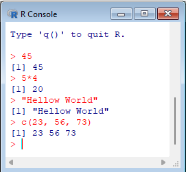 |
|---|
The R language works like a command line console. To print a string, simply type the string, also in quotes. It's an interpreted language, so it doesn't have to be compiled, nor is there an executable file generated; the R program itself reads the instructions and executes them.
The last instruction above builds a vector of elements, which is returned.
Action: | Expected: |
> # assigning values to variables | 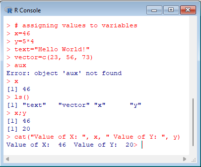 |
|---|
Comments in R start with # and continue to the end of the line. Notice the attempt to declare the aux variable, without the assignment. It doesn't make sense in R. Also note that the type of the variables is not specified. The ls() function lists all the objects that are defined. In this case it's only the x, y, text and vector objects, since the aux object hasn't been created.
The rm(<object>) function allows you to remove an object. When you exit the application, using q(), you can save the working environment so that you can continue later. The penultimate command is actually two commands on a single line. To separate two commands on one line, use a semicolon. In this case, the values of the variables x and y have been requested.
To get a result more similar to printf in C language, you can use the cat function, which must intersperse strings with variables.
You can redirect R's input and output with functions source(<file with commands>) and sink(<file with output>), but it's just as easy to insert the commands in a text file and simply copy/paste them into R so that the commands are executed.
The files are read/written from the directory in which R is run from.
Action: | Expected: |
> year <- 1345
> if(year%%4==0 && year%%100!=0 || year%%400==0) "Leap" else "Common" | 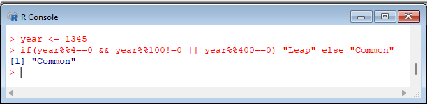 |
|---|
Conditionals can be used in much the same way as in C. The division remainder operator is %%, and the integer division is %/%. The logical operators in C and R are the same.
In the R language, it doesn't make sense to know the size of variables, as it is a loosely typed language. In this type of language, the memory occupied by a variable or data structure should not be the programmer's concern. However, there are basic variable modes in R: numeric; complex; logical; character. To obtain the basic mode of a variable, use the mode(<object>) function.
Action: | Expected: |
> sum=0; i=1
> while(i<=4) { sum=sum+i*i; i=i+1 }
> sum | 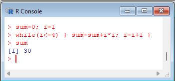 |
|---|
Action: | Expected: |
> Leap <- function(year) year%%4==0 && year%%100!=0 || year%%400==0
> Leap(2344) | 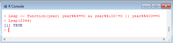 |
|---|
The definition of a function in R also consists of assigning an expression like:
function(<arguments>) expression
The expression can have a block of instructions, so that it can contain more than one command.
Once a function has been defined, it can be used inside other expressions.
Action: | Expected: |
> sum<-0
> for(i in 1:4) sum <- sum+i*i
> sum | 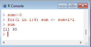 |
|---|
Action: | Expected: |
> 1:4
> c(1,2,3,4) | 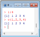 |
|---|
In R, there is also the repeat loop followed by an expression, which has no exit condition. The output of the cycle must use the "break" instruction, which exists in R with the same meaning as in C, and the "next" instruction is equivalent to "continue" in C. Usually, it is not advisable to use this type of instruction in either C or R, so the cycles to use should be the for and while loops.
Action: | Expected: |
> vector <- c(12, 45, 66, c(23, 455, 6)) > vector > sum(vector) > mean(vector) | 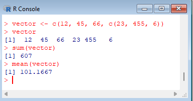 |
|---|
Action: | Expected: |
> vector[1] > vector[vector>25] > vector[vector>25] <- 0 > vector | 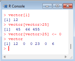 |
|---|
Action: | Expected: |
> matrix <- array(0, dim=c(10,10)) > matrix > matrix[,1] > matrix[1,] | 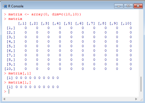 |
|---|
The array visualization shows the column and row headings, and also reveals a simple notation for extracting part of the array. The index [,1] returns a vector with the first column of the array, while the index [1,] returns a vector with the first row of the array.
3. Task 3: Structuring data to train a learning method
Learning methods require information to be structured into elements/observations/cases/instances, and each observation must have characteristics/indicators/properties that are measured. You want to know the classification (or the estimation of an indicator) of an element based on its features. The variable you want to know can be binary, discrete or real. We will focus our examples on binary variables, as this is the purest case of learning. For the sake of ease and affinity to statistical methods, we can call independent variables the characteristics/indicators/properties, the dependent variable what we want to know, and observations the elements/observations/cases/instances.
For supervised learning methods to work, there must be past observations with classifications, so all the independent variables and the value of the dependent variable must be known, and a given method can be trained to classify unseen observations. This information can be in the form of an array, with the independent variables in columns and the observations in rows.To load into R, we can place the data in a .csv file and read it (data.csv):
Action: | Expected: |
> setwd("set working folder") | 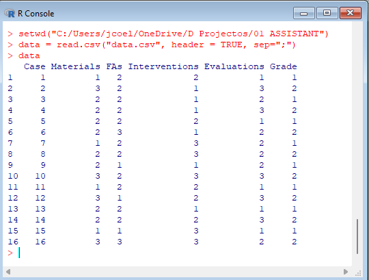 |
|---|
Action: | Expected: |
> data[,2:5] > data[,6] | 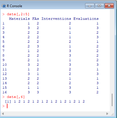 |
|---|
4. Task 4
Decision trees, K nearest neighbours, Neural networks
4.1. Task 4.1: Decision Trees
Documentation: randomForest function - RDocumentation
Action: | Expected: |
> install.packages('randomForest') | 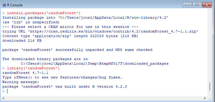 |
|---|
Action: | Expected: |
| > # ensure that the data is discrete (c.c. are considered linear)
> for(i in 2:6) data[,i]<-factor(data[,i])
> test <- randomForest(x=data[,2:5], y=data[,6], ntree=1, importance=TRUE)
> print(test)
> getTree(test, 1) # shows tree information, must be drawn
> test$type # confirm that it was a classification and not a regression
> predict(test, data[,2:5]) | 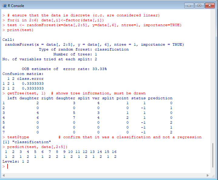 |
|---|
Action: repeat with training and test sets
4.2. Task 4.2: K nearest neighbours
Documentation: knn3 function - RDocumentation; knnreg function - RDocumentation
Action: | Expected: |
> install.packages('caret')
> library('caret')
> test <- knn3(x=data[,2:5], y=factor(data[,6]), k=3) > print(test) # shows number of cases for each value > predict(test, data[,2:5]) | 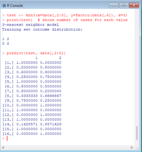 |
|---|
Action: repeat with training and test sets
4.3. Task 4.3: Neural networks
Documentation: nnet function - RDocumentation
Action: | Expected: |
> install.packages('nnet')
> library('nnet')
> # subtract 1 from y to ensure values are between 0 and 1
> test <- nnet(x=data[,2:5], y=data[,6]-1, size=1)
> print(test)     # network detail (weights) isn't shown
> test$wts        # weights
> predict(test, data[,2:5]) | 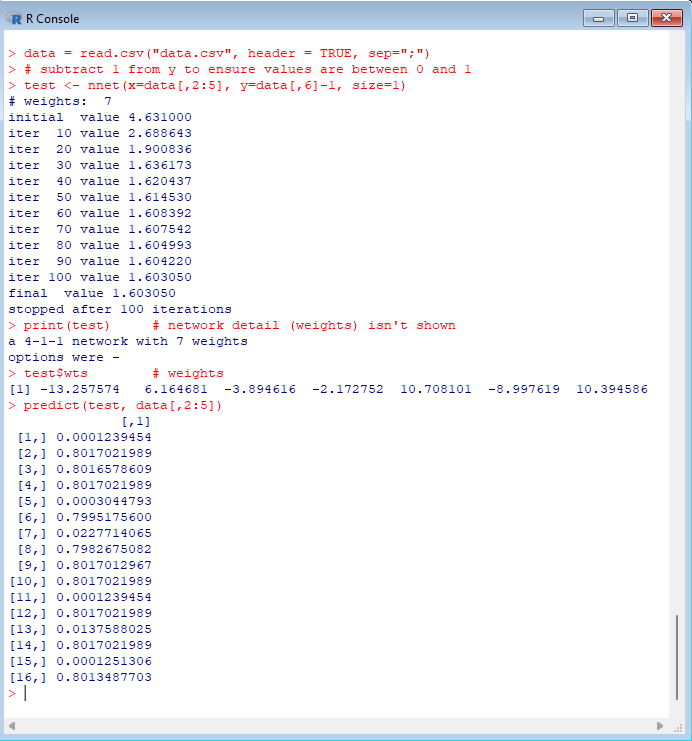 |
|---|
Action: repeat with training and test sets